EXCEL TUTORIAL (Beginners' Guide)
The essence of this tutorial is to take the
reader (you) through the basics of Microsoft EXCEL as a form of spreadsheet
package used to input and calculate numerical data.
Learning Goals:
- Identify an Excel icon in a desktop application.
- Use Excel worksheet in calculating simple numerical
problems
- Editing cell content(s)
- Save and Print an Excel document in a named file.
An Excel
worksheet can be opened by double-clicking the icon if available on the Windows
Desktop. Otherwise, click the start Menu and select program(me). In most cases,
this can be found by pointing the mouse to MS Office sub-menu and then select
Excel.
The diagram below illustrate a typical Excel
application window when an Excel icon is clicked:
Table
1
![]()
 Active Cell Column Scrollbar
![]()
![]()
![]()
Row
Formula Bar
An excel application window consists of Rows
and Columns and these are identified by a unique cell number. For example, the
bold print rectangular active cell box from the diagram above consists of a
unique cell number- A1. Other important part of an Excel application window
include:
Formula Bar- this displays all formula entered on an
active window.
Scrollbar- this is used to move an Excel worksheet
from top to bottom of the page.
Data Entry- Information
entered on an Excel worksheet is referred to as data. As explained
earlier, these can be entered in the cell by pointing the mouse on the
particular cell in which the data is supposed to be entered. This will now be
the active cell, which is indicated by a bold print as shown in the rectangular
shaped cell.
Types
of Data Entered on an Excel Worksheet
- Text- this can be a letter or any character
other than a number. In most cases, text data can be used to name the
worksheet (indicated in the head of the sheet) or to identify variable(s)
used.
- Number- this can take any value and in some
cases, can be combined with currency or a point to specify a decimal
number. Numbers written on an Excel worksheet always bear a unique cell
number identified by the particular row and column in which it is placed.
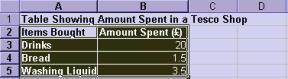
For example, suppose you want to list the items bought on a Saturday at
Tesco Supermarket, this can be entered in an excel worksheet as shown
below.
Table2
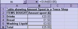
Total amount spent
from the above table can be calculated by adding up all the ‘Amount Spent’ in
column B downwards. In short the total can be calculated by using the formula
“=B3+B4+B5” or SUM(B3:B5) in the formula bar in Table 2. This means summing up
all values from column B3 up to B5.
Notations
used in Excel Formula
Type Notation/Symbol
Addition +
Subtraction -
Multiplication *
Division /
Greater than or
equal to >=
Less than or equal
to <=
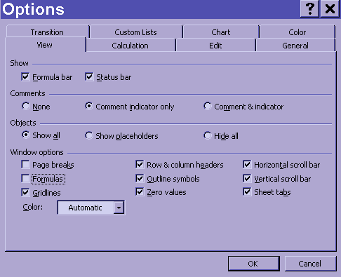
SHOWING
FORMULA
Dialogue
Box to display Formula
|
Table 3
|
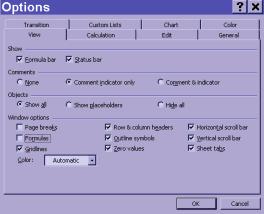
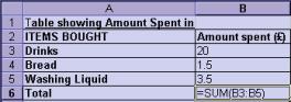
Steps to show formula:
- Highlight the particular row or column in which you want
formula to be shown.
- Click the Tools menu and select the option sub menu.
- Tick off the formula option box as indicated by bold
rectangular box in the Dialogue Box above.
- This will automatically be shown in the worksheet as
indicated in Table 3.
CHARTS
A chart can be
defined as a graphic representation of data from a worksheet. Values inputted
in the Excel worksheet can be illustrated by charts of all sort for example,
Graphs and Pie Charts. A simple way of doing this is by selecting or
highlighting the data to be represented in the graph and then click the Chart
Wizard icon as shown in the standard Toolbar box. Alternatively, this can be
done by clicking the Insert menu and then select chart.
Table 4 Graph Produced from Table 4
|
|
|

There are four
steps involved in creating a graph from an Excel worksheet table. The first
step is to select the type of chart needed (i.e., whether Graph or Pie Chart)
after clicking on to the Chart Wizard Icon. The remaining steps involve naming
the chart and the different axis present. For example, Amount Spent from
table 4 above is represented on the Y-axis (Vertical) and Items on the X-axis
(Horizontal).
Adding
Rows and Columns to an existing Excel Worksheet
This can be done by
highlighting the particular row or column where the insertion should take place
and then click on to the Insert menu and then select row or column which ever
is needed.
Editing
Cell Content
Cell content in an
Excel document or worksheet can be edited by highlighting the particular area
in the document to be edited. For example, a number can be changed by simply
deleting the content of the cell and replace it with the new number. The
advantage of using Excel spreadsheet is that, any changes made to an existing
document can automatically be adjusted. For example, increasing the amount
spent in Bread will automatically adjust the Total.
Also, a whole Excel
worksheet can be copied on to another worksheet by highlighting the entire
document and right click the mouse and select ‘Copy’. This can then be pasted
on a different worksheet by right-clicking the mouse and then select paste.
This will finally placed the worksheet copied from the previous sheet on to the
new sheet.
Saving
and Opening an existing Excel Document
An Excel document
or worksheet can be saved by clicking on to the File Menu and select Save As
for a new document.
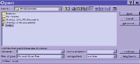
Save As Dialogue Box Open
Dialogue Box
|
|
|
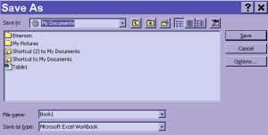
To provide a name
to an Excel document, specify the location in which the document should be
saved by clicking the save in box as shown above. If you want the file to be
saved in a floppy disk, then select the 3.5 floppy option. The document can
also be saved in the C drive by clicking the C: option. The second stage is to
provide a name to the file by clicking in the File Name box. The document can
be saved in an older version of Excel by clicking in the ‘save in type’ by as
shown above. Clicking this will produce a drop down list of Excel versions,
that is, Excel 5,6. After completing all of the above steps, then click the
save box which will finally the save the document in the name selected.
Similarly, an
existing Excel document can be opened by clicking the File Menu and then select
Open. If the file is saved in a floppy disk, then select the drive by clicking
on the ‘look in’ box as can be seen in the Open Dialogue box. This will
then display lists of files already saved in the floppy disk or the C drive.
After completing all of these, then click the ‘Open’ box to open the
particular document selected.